Headline
One of the annual review digests back in 2020 stated that executing Kerberoasting attack as part of internal penetration testing routine results in 61% success. This fact inspired me to untangle the attack, looking for answers to why is Kerberoasting so popular, what are the existing protection approaches, and which of them are currently in use.
Before discussing the attack itself, it is essential to have a general understanding of how Kerberos authentication works.
Authentication
The following tools are involved in Microsoft authentication over Kerberos:
- Key Distribution Center (KDC) — one of the Windows Server security services running on a domain controller (DC);
- A Client that attempts to authenticate and access the service;
- A Server, which a user attempts to access.
The Client and the DC communication scheme can be represented as a message flow:
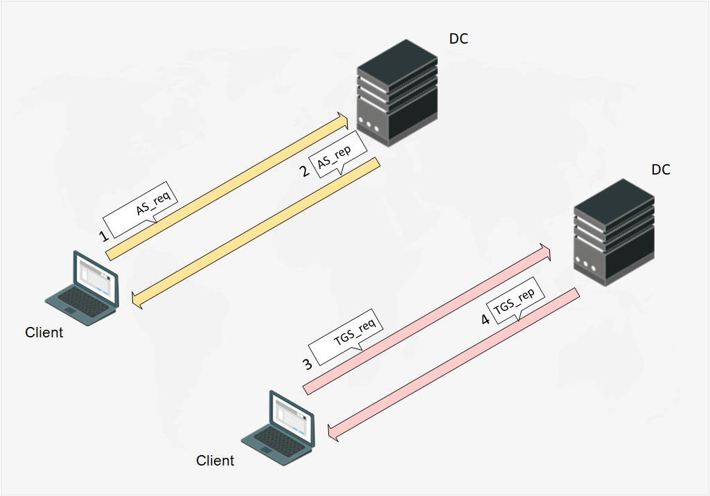
Fig. 1 The Client and the DC message flow scheme
AS_req
When the Client starts authentication, it sends a message AS_req (Authentication Service Request) to the DC. The AS_req-message includes UPN (UserPrincipalName), accessed service name (always krbtgt), and a timestamp encrypted by the user account password hash.
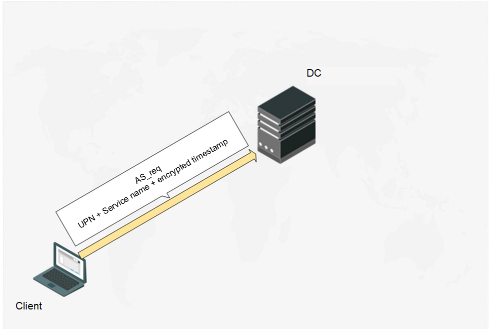
Fig. 2 The Client starts pre-authentication
The ASreqroasting attack is based on the latter. Executing MITM-attack, an attacker can intercept AS_req-message to extract the encrypted timestamp from it and implement brute force passively via hashcat (mode 7500 if timestamp is encrypted by RC4 or mode 19900 if timestamp is encrypted by AES256). For exploitation details refer to this link. ASreqroasting attack is less popular comparing to other Kerberos roast attacks, though it has being known since 2014.
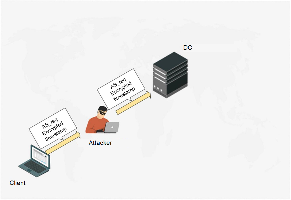
Fig. 3. The attacker exploits MITM and intercepts the AS_req message
AS_rep
When the DC obtains AS_req-message, it first decrypts the timestamp by the user password hash. If the encrypted timestamp difference from the current time exceeds 5 minutes (Time Skew parameter by default), the PreAuth failed answer will be sent. When a timestamp is decrypted, the DC sends the AS_rep (Authentication Service Reply) message in reply. The AS_rep-message contains TGT (Ticket Granting Ticket), encrypted by the krbtgt account password hash and session key encrypted by the user account password hash. TGT ticket can also contain the same session key. The session key is required to encrypt subsequent message from the Client to the DC.
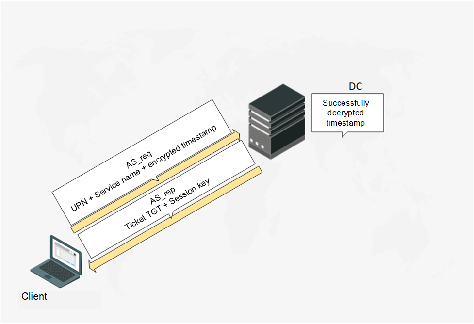
Fig. 4. DC sends the AS_rep message in response
And again the roast-attack can be executed here. The point is that timestamp signing in the AS_req message can be disabled for the user account (disabling Kerberos pre-authentication). This means that the attacker can enumerate the accounts with disabled pre-authentication and send AS_req message to the DC on their behalf. In reply they will receive the AS_rep message. As we know, this message contains a session key encrypted by the user account password hash. This attack type is known as ASREProasting. Though there are only a few cases when pre-authentication has been disabled, this attack has a number of advantages:
- Can be applied without any domain account (network access to DC is enough), although enumeration of user accounts with disabled pre-authentication may pose a problem;
- The received hash may be iterated over in passive mode the same way as in ASreqroast (hashcat mode 18200).
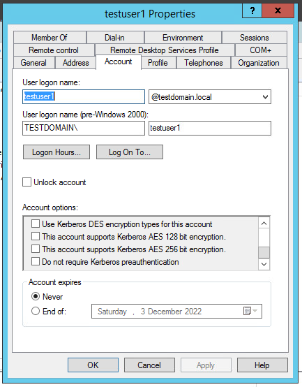
Fig. 5. Disabling pre-authentication
TGS_req
After passing pre-authentication, the Client sends DC a TGS_req (Ticket Granting Service Request) with the following content:
- SPN (Service Principal Name) — service name to which the Client requests the access. It is associated with either a computer account or a user account;
- UPN and time stamp encrypted by earlier obtained session key;
- TGT ticket.
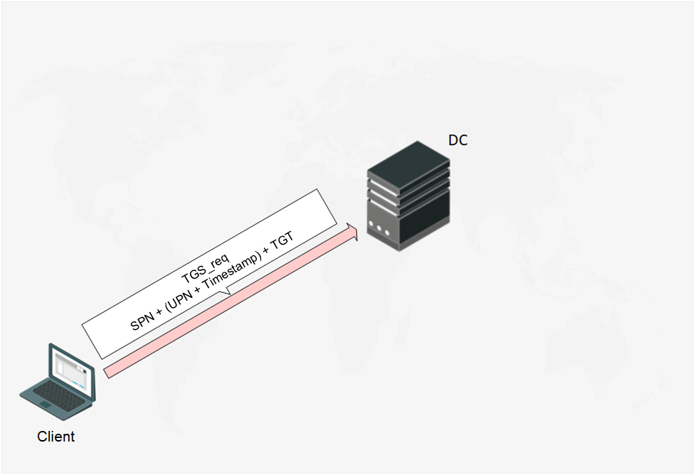
Fig. 6 The Client sends the TGS_req message
TGS_rep
After the DC receives the TGS_req-message, it validates the SPN and TGT ticket validity period (TGT ticket validity period is 10 hours by default), decrypts, and analyzes the timestamp. If the SPN is correct, the TGT ticket validity period is not expired and all timestamps are within the valid range, then the DC will send the Client a TGS_rep (Ticket Granting Service Reply) message containing a TGS (Ticket Granting Service) encrypted by the password hash of the account used to launch the service. And this final part is what makes the Kerberoasting attack possible.
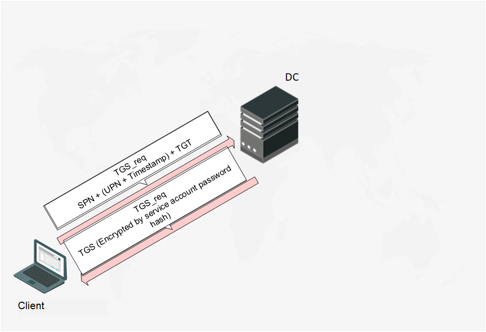
Fig. 7. Client obtains TGS ticket
Afterwards the AP_req and AP_rep messages will be sent for Kerberos authentication. There is little use describing them here since the given explanation should be sufficient for understanding the attack.
Kerberoasting
There are two reasons why Kerberoasting is possible. First, the DC does not authorize the Client, so the DC cannot grant the Client permission to access arbitrary services. Using a single domain account the attacker can create a legitimate TGS ticket request to all SPNs in the domain. The attacker is interested in the SPNs associated with user accounts rather than computer accounts due to the pointlessness in retrieving passwords of the latter. Second, TGS tickets are encrypted by the service account hash. This will help the attacker to retrieve the service account password if the password is not strong enough.
The attack can be divided to a number of stages:
- The attacker begins authentication in a domain (AS_req and AS_rep).
- The attacker uses a TGT ticket to request TGS ticket receipt for a specific SPN (TGS_req and TGS_rep).
- The attacker extracts the hash from the encrypted TGS ticket from the TDS rep.
General facts about the attack:
- Easy to exploit. There is a wide variety of instructions on how to enumerate SPN requests to obtain TGS tickets, how to perform all the actions in parralel by using Impacket GetUserSPNs.py module etc.
- To launch the attack, it is sufficient to have a domain account with any privilege level plus network access to DC over UDP/88;
- Obtained service account hashes may be iterated over in passive mode.
The attack is often used by white hats and black hats alike. An offended participant of the Conti partnership program published a hacking group’s tutorial where Kerberoasting was described as one of the main attacks. The guide recommended to attempt Kerberoasting as the first option when attacking a domain.
Example of the attack exploitation by means of GetUserSPNs.py:
ntpdate 10.23.53.26; GetUserSPNs.py -request -dc-ip 10.23.53.26 TESTDOMAIN.local/testuser1:Testuser! > kerberoast.txtwhere:
- ntpdate — time synchronization of a malicious actor computer with DC time. It is highly possible to get an error KRB_AP_ERR_SKEW(Clock skew too great) without this command;
- 10.23.53.26 — DC IP address;
- GetUserSPNs.py -request -dc-ip — running a script with options -request and -dc-ip;
- TESTDOMAIN.local — domain name;
- testuser1:Testuser! — domain account login and password;
- > kerberoast.txt — recording of script output GetUserSPNs.py to a text file.
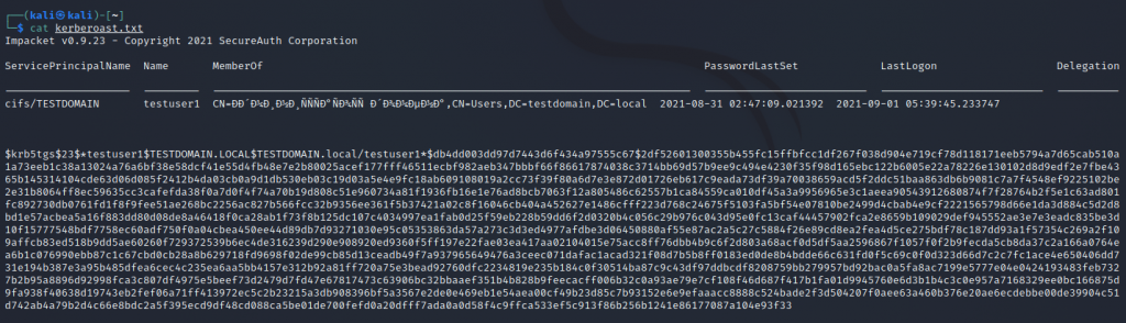
Fig. 8. Output of kerberoast.txt
Then, hash will be iterated over and if the password is not strong enough, the attacker will be able to guess the password for the service account.
Countering the attack
1. Strong password policy and reduced service account privileges
The simplest way of protection is to set all passwords belonging to service accounts to be 25–30 character long and to ensure that all service accounts are given only essential privileges, for example, the service accounts should not be included in the domain administrator group. It sounds quite simple, but unfortunately, Kerberoasting effectiveness shows that usually these recommendations are not followed.
2. An SPN honeypot
Another efficient approach to detecting Kerberoasting. It involves creation of an unusable account and an SPN (the SPN created is not associated with any real application). Kerberos clients would never request a TGS ticket for a false SPN, therefore, if a 4769 event appears in the DC security log for this service, the Kerberoasting attack will be detected.
Example of a 4769 event (TGS ticket request), alerting that Kerberoasting attack is underway.
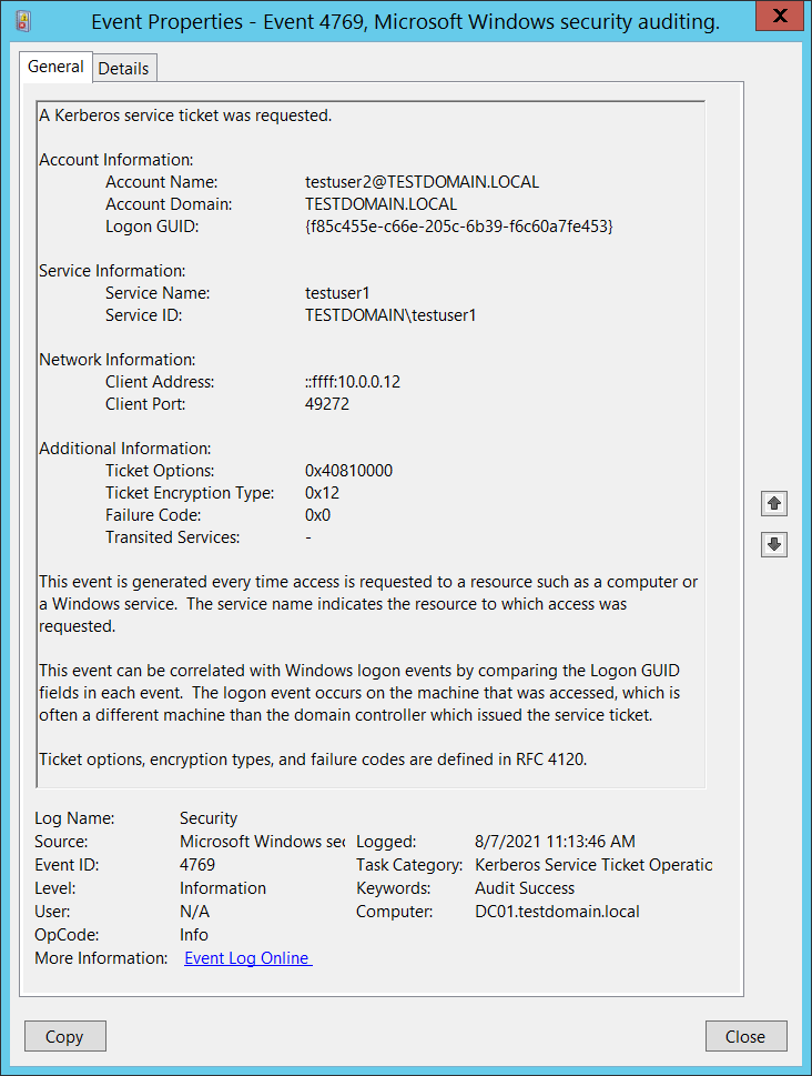
Fig. 9. 4769 events indicating that a TGS ticket has been requested for a non-existent service
In this event:
- Testuser2@TESTDOMAIN.LOCAL — the compromised account used by the attacker to request a TGS ticket;
- Testuser1 — a trap account. A false SPN is associated with this account;
- 10.23.53.29 — the ip address used for attack.
Therefore, security team can detect the fact of the attack and identify the source computer.
3. FAST (or Kerberos armoring)
Flexible Authentication Secure Tunneling (FAST) or Kerberos Armorin is a DC security configuration that establishes a protected channel between the Kerberos client and the KDC within AS_req, AS_rep, TGS_req and TGS_rep messages. It is supported by Windows Server 2012 and Windows 8 and up. Detailed approach description is provided in RFC 6113 and RFC 4851.
Here’s a description on applying Kerberos Armoring:
- Enable Kerberos Armoring support on the DC. Open Group Policy Management, proceed to Default Domain Controllers policy, right-click to open context menu, select Edit. Select Computer configuration → Policies → Administrative Templates → System → Key Distribution Center. Open KDC support for claims, compound authentication and Kerberos armoring on the right part and set up Enable, enable Fail authentication requests when Kerberos armoring is not available.
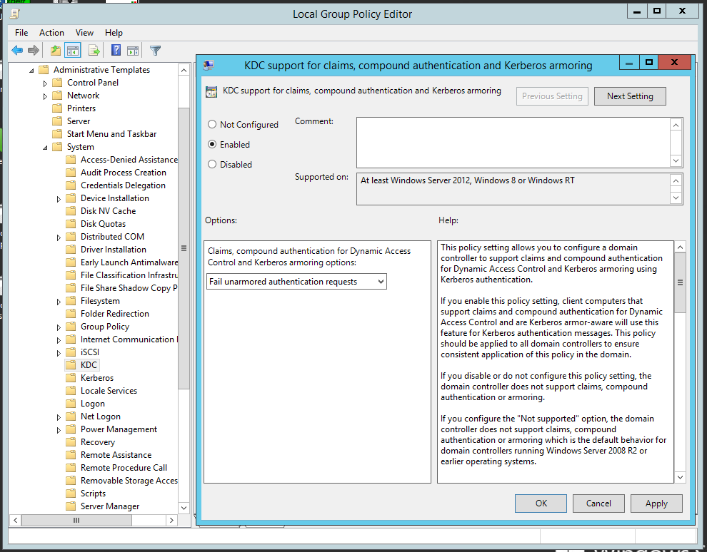
Fig. 10. Enabling Kerberos Armoring support on the DC
2. Enable Kerberos Armoring support for the Kerberos Client. Open Group Policy Management, proceed to Default Domain Controllers policy, right-click to open the context menu, select Edit. Then select Computer Configuration → Policies → Administrative Templates → System → Kerberos. Open KDC support for claims, compound authentication and Kerberos armoring on the right part and set up Enable.
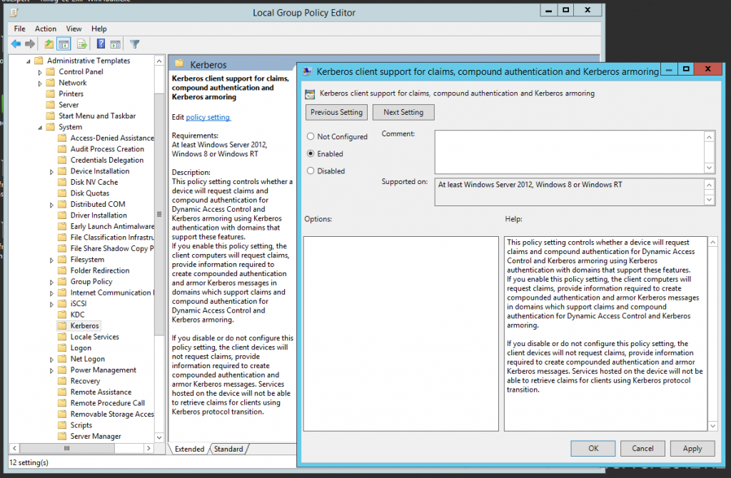
Fig. 11. Enabling Kerberos Armoring support on the Kerberos Client
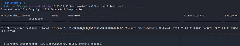
If we care to intercept the Kerberos message by Wireshark, we will be able to see the error NT STATUS: Unknown error code 0xc00002fb:

For a detailed description of the error 0xc00002fb: An invalid request was sent to the KDC, refer to the link.
The DC refused the attacker in pre-authentication because it is expecting secure channel to send AS_req and AS_rep messages.
4. gMSA
Group Managed Service Accounts or gMSA represent the type of accounts in AD used for secure service start up. A 240-character password will be generated for each gMSA and by default it will change every 30 minutes. The password is managed by the AD and is not stored in the local system, therefore, it cannot be extracted from the LSASS process dump. gMSA authentication relies on Kerberos only. It is supported starting from Windows server 2012. For more details refer to the link.
An example of gMSA setup:
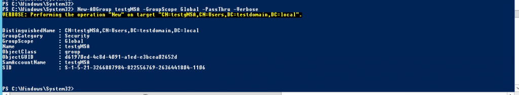
- Create a server domain group with a permission to use group service account:
New-ADGroup testgMSA -GroupScope Global -PassThru -Verbose
where testgMSA is a name of the created domain group.
Next, add a server (i.e. WIN-D300I3D4GHE) to the testgMSA group:
Add-AdGroupMember -Identity testgMSA -Members WIN-D300I3D4GHE$
2. Сreate a gMSA group account:
New-ADServiceAccount -name gmsa -DNSHostname gmsa.testdomain.local -PrincipalsAllowedToRetrieveManagedPassword testgMSA -Verbose
where gmsa is the managed service account for the created group.

3. Enable the gMSA account on the server added earlier (in our case it would be the WIN-D300I3D4GHE):
Install-ADServiceAccount gmsaInstallation is possible only if gmsa is implemented on the server:

4. The last step is starting up a service on the gMSA behalf.
This way we can start up services on behalf of gMSA account, making password retrieval impossible, even in cases when the attacker has managed to obtain an encrypted TGS ticket hash.
By Yuri Chernishov, Head of R&D Center
Introduction
In our world new things appear daily. New knowledge domains that were never thought of just several years ago, appear on a regular basis while old domains disappear, unable to sustain competition. Each knowledge domain is defined by specific knowledge that describes domain objects and their properties. Practical use of this knowledge is maintained by the experts. Even more, professional competencies of the experts are defined by possession of specific knowledge although rapid changes in technological innovation make obtaining wide and deep expertise a challenge. One of the reasons behind this is the huge amount of data generated by each and every subject domain and industry.

Contemporary observations show that the growth of data amount has become exponential, in other words, the growth rate of data amount depends on the current data amount linearly. The more data there are, the higher becomes the rate of the data amount growth. The importance of this trend can hardly be overestimated – both technologically and psychologically. Enormous amounts create difficulties in data transfer, processing and storage, despite significant increases in hardware performance. Yet, the true challenge lies not in the mere amount of data, but rather in the fact that the data has no structure. Data are provided by different sources, in various formats and at different time periods. In order to store and use these data in practical tasks preprocessing is aimed at making the data structured and converting it into suitable formats. A traditional way to store and use data is based on relational databases where the data are stored in relational tables. However, in many cases use of tabular data is ineffective. As the result, alternative forms such as Knowledge Organization Systems (KOS) have been developed. Their use is based on knowledge graphs.
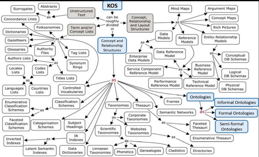
Various structures are used to store knowledge:
- Controlled vocabularies: knowledge arrangement method for subsequent search implemented in subject indexing schemes, subject entries, thesauruses, taxonomies and other KOS.
- Thesauruses: merge terms into groups by a specific property such as resemblance (synonyms).
- Taxonomies: categorized words organized by a hierarchical trait.
- Ontologies: description of formal knowledge from a domain (subject domain) considering existing complex rules and relations between elements that allow automatic knowledge extraction (reasoning).
- Datasets: machine-readable data sets.
Ontologies are developed for Knowledge Organization Systems and are essential in spheres where detecting new facts and identifying hidden relations between components (for example, recommender and expert systems) are imperative. This is an alternative to classic databases where “closed-world assumption” is implemented, in other words, it is assumed that everything that is not included into the database does not exist. In contrast, “open-world assumption” is adopted in ontologes where we assume that if a knowledge base does not include something, it does not mean that it does not exist. It rather means that it has not been described yet.
Knowledge organization systems are widely spread and implemented in many industries. A striking example is a knowledge graph developed to search information in the Internet. It has considerably improved search quality. Some other ontology implementation examples include:
- Banks use knowledge graphs for fraud detection.
- Graphs based on legal documents are usually implemented in consulting.
- Aggregated data based on patient health is used in healthcare, Health Electronic Record.
- Knowledge graphs are implemented in various industries for supply-chain management. In fact one of the main features of the Industry 4.0 is the interaction of cyberphysical systems that leads to automation and demands some form of knowledge management.
- Knowledge bases are often used to manage chat-bots as well as to process complex queries in natural language (for example, asknow service).
- Ontologies are also applied in a wide range of natural language processing tasks: text annotation by means of ontologies, knowledge extraction, NER, Named Entity Linking, Relation Linking, automated new knowledge deduction, reasoning. SemTech solutions see rapid development all around the world as well.
Ontologies are also applied in information security. Installing patches and updating software in order to decrease attack possibility will never provide a 100% protection due to vulnerabilities caused by insecure user behavior and infrastructure configuration, errors in implemented security tool configurations, password configurations and insufficient privileged access control. Protection from zero-day attacks is extremely difficult as well, as no rules exist that would detect this attack type, both recognition and response are supposed to take place on the fly. One way to recognize an attack with an unknown pattern is to use accumulated knowledge and reasoning taking into account all available information on current events. Such knowledge can be stored by means of ontologies where the data about correlations between various entities are stored.
What are ontologies?
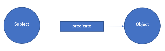
Ontology is mathematically based on the so called description logic (a branch of mathematics) that assumes that any information expressed in a natural language can be represented as triplet series.
A passage from an English nursery rhyme “The House That Jack Built”.
…
This is the rat,
That ate the malt
That lay in the house that Jack built.
…
The relations between different entities described in the rhyme can be represented as an ontology.
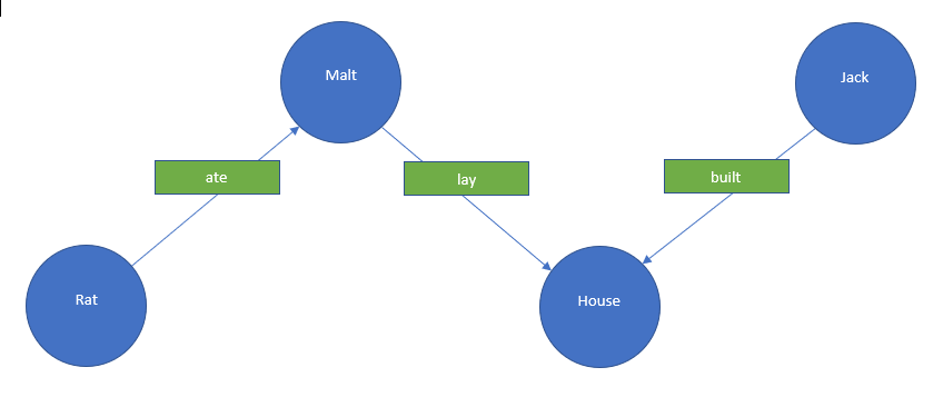
The ontology is represented as a graph where the nodes are entities and the arches are relations between the entities. It is deemed that any statement in natural language can be represented as simple sentences and entities as well as relations between these entities can be extracted from the sentences. There are two main tools: RDF (Resource Description Framework) or OWL (Ontology Web Language). One of the OWL features is support for descriptions for the logical rules for the data. Ontologies (in contrast to standard databases) help find hidden data. Standard ontologies are applied when a search for specific information is required and knowledge bases are intended to identify new knowledge, for instance, in decision support systems (expert systems).
RDF store examples: Virtuoso, 4store, stardog.
Ontology is particularly useful when a detailed and thorough description of the relations between the components is provided by means of a mathematical tool of descriptive logic. For example, properties can be assigned to relations (functional, transitive, reflexive). As a result, facts are automatically extracted from ontologies; this process is defined as reasoning. There is a variety of reasoning algorithms based on graphs. Here are some examples of application options: refining object characteristics and extraction of a unique object from a set of similar objects, search for similar objects, “text understanding” and text classification, assistance in NLP tasks (NER, Relation Extraction), root cause analysis, pattern detection. There is a wide variety of tools that support reasoning such as as IBM Watson, Wolfram Alpha. However, the most popular editor is Protégé.
Ontologies are usually created manually by professionals. Though, there also are examples of automatic ontology creation based on existing knowledge bases. Open-source knowledge graphs (at the end of 2021, according to data provided by https://lod-cloud.net/:
- DBpedia
- Yago + wordnet.princeton.edu
- WikiData
- Open-source knowledge base including object and industrial knowledge bases, for example, healthcare: BioPortal, Bio2RDF, PubMed
The tools above provide various methods for operation with ontologies, however as the most popular tool is Protégé, we shall base our further discussion on its logic and features.
Working with Protégé
Installation
Protege is designed by Stanford University to develop, edit and use ontologies. The software is free and can be downloaded from https://protege.stanford.edu/products.php; web version is also available on https://webprotege.stanford.edu/ and an archive file is provided on the official page for using it on a local computer. It is important to account for the operating system and processor architecture (64-bit or 32-bit). The latest Protege version (at moment of writing this) is 5.5, however, legacy 32-bit operating systems would require older Protégé versions, such as Protégé 4.3.
Extract Protégé.exe file to any folder and start it. Now you can create ontologoes. But it is just the beginning of a long and arduous journey, but an interesting one.
Project creation
When the program starts the following window opens.
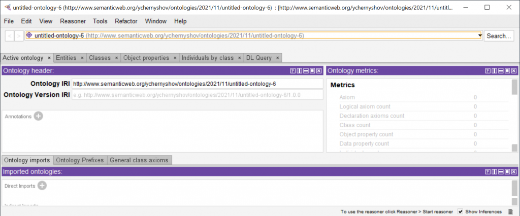
Everything is in English and Java here, but English is actually enough for understanding.
Each project has a unique identifier – IRI (Internationalized Resioure Identifier).
Protégé allows to record triplets represented as “subject-predicate-object”.
The Entities section allows describing subjects and objects.
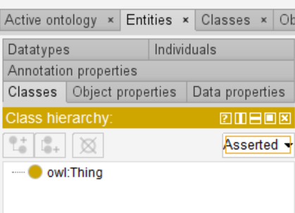
Important tabs in the section:
- Class instances (Individuals). The same class objects as in object-oriented programming. For example, the “Server” class, “prod-serv-002” object.
- Properties (object properties or data properties). Similar to class properties in object-oriented programming. However, in ontologies properties are independent and can be separated from the class (unlike object-oriented programming).
Various properties can be assigned to predicates, i.e.:
- Functional
- Reverse
- Transitive
Reasoner can be applied to the described ontology. It makes offers based on the obtained facts (which can be accepted or rejected).
Ontologies can be saved as an owl file and look exactly like a typical xml file if opened in a text editor.
It will be easier to explain these concepts on examples.
Practical tasks for Protégé
Personnel access to rooms
Let’s imagine a situation in which we need to track the location of each employee. We know that:
- Johns does not have access to the server room and the room 101.
- Hansen does not have access to the 101 room.
- Smith does not have access to the document storage room.
There are three employees (Johns, Hansen, Smith) and three rooms (the server room, room 101 and the document storage room). For a clear-cut solution, ontology component properties must be strictly defined, for instance, establishing the fact that there are no other employees and rooms and that one employee has access to only one room otherwise it will be impossible to logically solve the task. If strict restrictions are set up, task solution will be trivial. The first condition implies that Johns has access to the document storage room (since the server room and the room 101 are excluded); Hansen (the server room and the 101 room are left) has access to the server room and Smith is left with the room 101. Now it will be easier to check operation results of the Protégé reasoner, which was trusted to solve the problem.
Start Protégé editor.

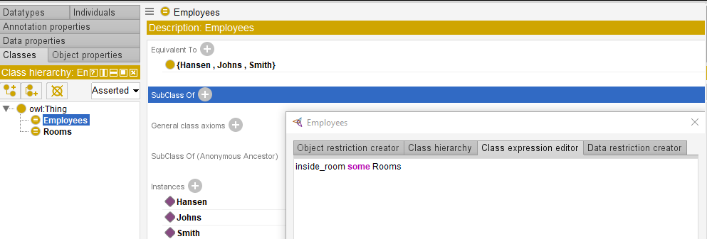
Now we can start creating an ontology for the task in the main window. At first, let’s create two classes: “Employees” and “Rooms”.
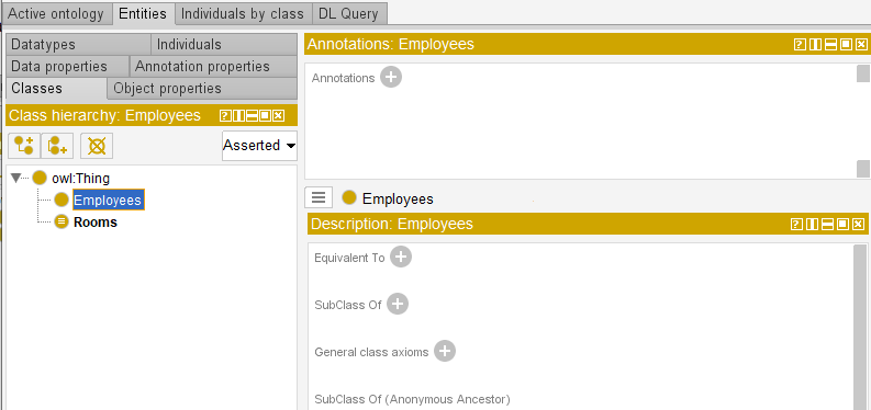
Let’s create instances for these classes.
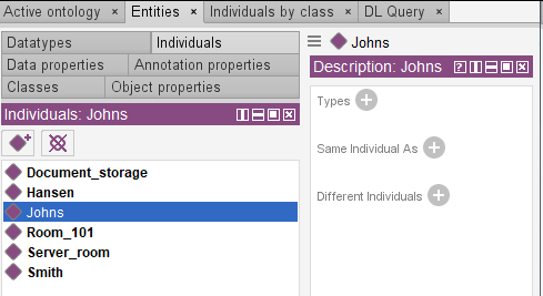
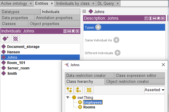
Let’s repeat this procedure for the remaining employees (Hansen and Smith) and the rooms.
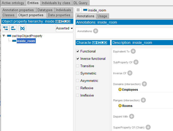
Now object property “inside_room” can be created. It will connect Employees and Rooms. When object property is created, entities related by the predicate should be specified. In our case they are Employees (Domain) and Rooms (Ranges). Employees can be in any room and a room can accommodate any number of employees. The property is functional and acts from the Employees domain to the Room range. Based on principles of biology and physics, one employee can be only at one room. This fact must also be taken into account when “inside-room” property is determined. Functional and Inverse parameters should be assigned to this property; as a result binary relation “one-for-one” will be formed.
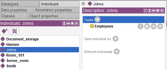
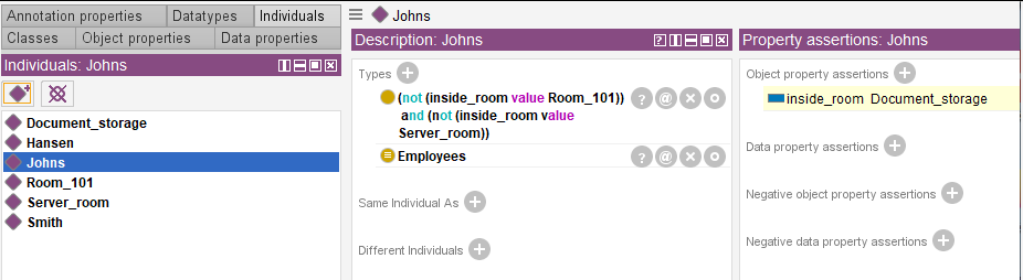
Let’s add known information on employee location to our ontology.

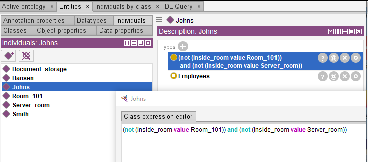
Let’s add similar information on Hansen and Smith using logical predicates “not” and “and”.
We can try to start a Reasoner.
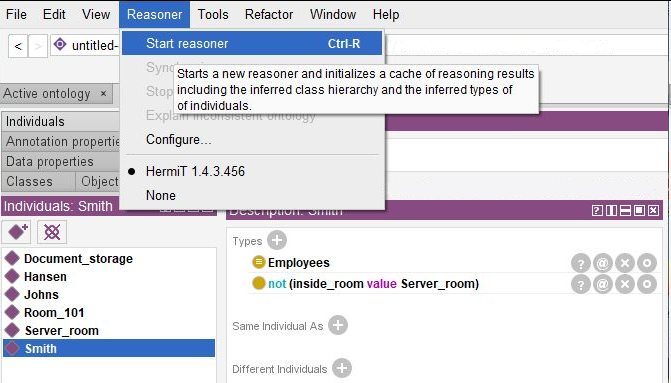
However, new objects (employees and rooms) still can be added to the current statement according to the open world hypotesis therefore no significant facts can be extracted. To conclusively solve the task referred to employee location detection, the reasoner requires strictly defined properties for “Employees” and “Rooms” classes.
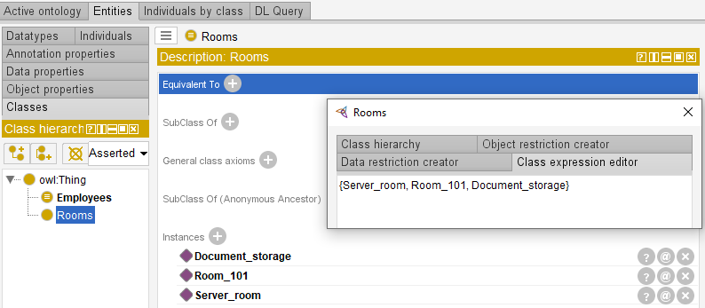
To establish one-to-one relations between the ontology entities it is required to specify that each employee must be at least in one room.
Starting (or synchronizing) the reasoner will provide information on the employee exact location in a certain room. For example, we have established that Johns is in the document storage room.
The selected ontology can be saved e.g. in owl format.
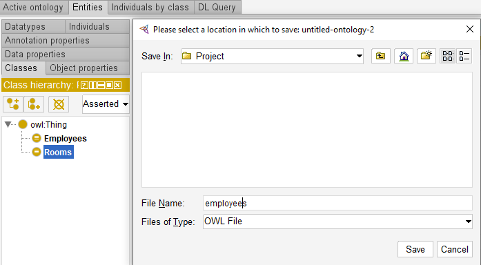
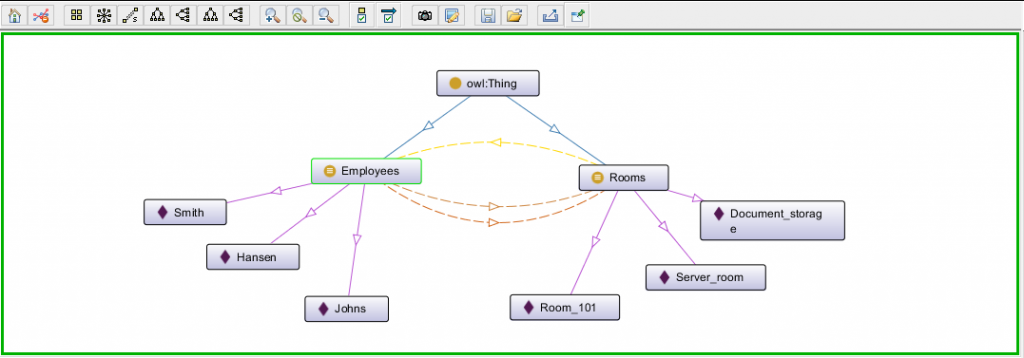
The obtained .owl file can be opened in any standard text editor. However, information is perceived better when represented in a graph and Protégé provides such option.
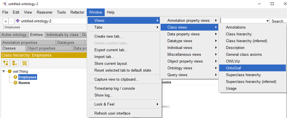
As a result, an informative visualization is generated.
As the described problem is quite simple one and can be solved by unsophisticated logical reasoning. The problem that we are going to discuss next is more complicated and only few people can solve it in their minds.
Einstein’s Riddle
Problem statement
An Einstein’s Riddle is a well-known logical puzzle. It consists of 15 clues meant to help in finding answers to the questions of who drinks water and who owns a zebra.
The original riddle text is as follows:
- There are five houses.
- The Englishman lives in the red house.
- The Spaniard owns a dog.
- Coffee is drunk in the green house.
- The Ukrainian drinks tea.
- The green house is immediately to the right of the ivory house.
- The Old Gold smoker owns snails.
- Kools are smoked in the yellow house.
- Milk is drunk in the middle house.
- The Norwegian lives in the first house.
- The man who smokes Chesterfields lives in the house next to the man with the fox.
- Kools are smoked in the house next to the house where the horse is kept.
- The Lucky Strike smoker drinks orange juice.
- The Japanese smokes Parliaments.
- The Norwegian lives next to the blue house.
Who drinks water? Who owns a zebra?
In the interest of clarity, it must be added that each of the five houses is painted a different color, and their inhabitants represent different nations, own different pets, drink different beverages and smoke different brands of American cigarettes. One other thing: in statement 6, right means your right.
Solution
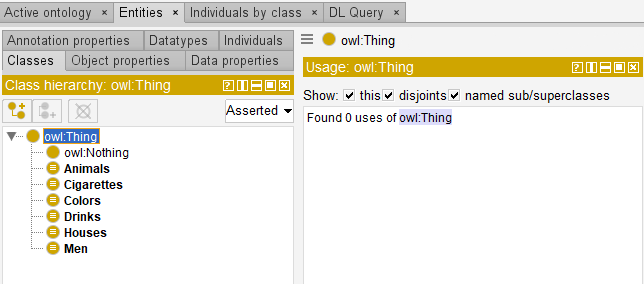
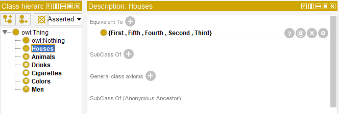
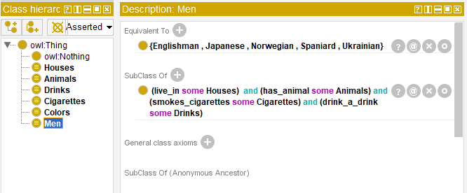
The first stage includes determining classes. There are five classes: “Houses”, “Men”, “Animals”, “Drinks” and “Cigarettes”. The “Houses” class has two features which are house number and color therefore it is reasonable to create a new class – “Colors”.
The next step is to create class instances (objects).
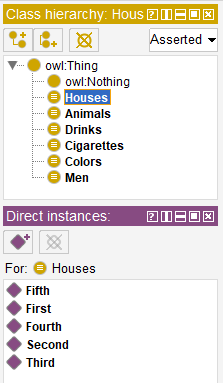
The rest five classes are subject to the analogous procedure.
Then properties for objects and object characteristics are to be created. Six properties (predicates) will be created in the “Object Properties” section: “live_in”, “has_color”, “has_animal”, “smokes_cigarettes”, «located_right_of», “drink_a_drink”. Entities related by predicates and their characteristics are to be specified in the process of predicate creation.
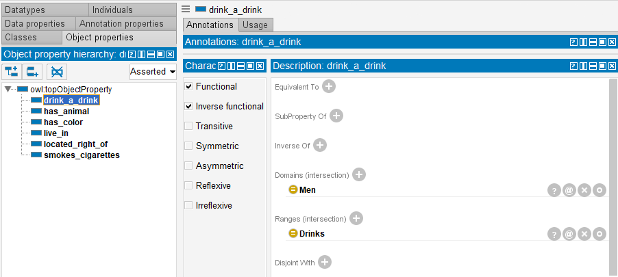
Let’s run the same procedure for the other predicates.
Functional and Inverse functional parameters are assigned to all six properties. It is a binary “one-for-one” relation.
Now it is time to add all known facts about entities to the ontology. The first fact is that the houses are in 1-5 order. For this purpose, we will specify that the “First” object is to the right of the empty set and that the “Fifth” object it is to the right of the forth house and to the left of the empty set.
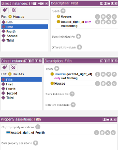
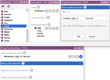
For the “Second”, “Third” and “Fourth” objects we should specify that they are to the right of the previous one in the “Object property assertions”.
It is also required to add information from simpler statements represented as triplets such as “Spaniard owns a dog”.
Next step is adding information contained in the riddle statements. Though, by the first look, this information does not help in searching for the answers required.
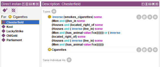
In the example above, service word inverse makes a cigarette brand the statement subject because Chesterfield is smoked by the man and not vice versa.
The information from other statements will be added in the same way. If we try and start the reasoner now, no significant facts can be extracted because all classes are open in the current statement and an option to add new objects is preserved. The reasoner will be able to solve the problem only if the classes are strictly determined.
The other five classes must be determined in the same way. To define the ontology the fact that each man definitely leaves in a house, drinks a drink, owns a pet and smokes the cigarettes of a certain brand must be indicated.
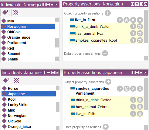
Starting the reasoner will provide us answers to the questions. Now we know that the Norwegian drinks water and the Japanese owns zebra.
Obviously, well-described ontologies can help solve difficult problems, however, it is required to meticulously describe properties of an ontology components, entities and predicates.
Conclusion
It is important to realise that ontologies implementation is not always efficient in solving problems. The solution method is to be determined based on subject domain particularities.
Various knowledge bases have already been created in information security such as MITRE ATT&CK and SHIELD, CVE, CAPEC. They are implemented in incident analysis and response, investigations and vulnerabilities detection. But let this be the topic of the next article.
The number of devices, systems, services and platforms belonging to industrial, informational and cyber-physical spheres arоund us increases daily. Usually, we do not bother thinking about how a coffee machine makes a cup of coffee, how a robot vacuum cleaner determines the best cleaning routes, how a biometric identification system identifies people on a video or government services portal processes our requests. Everyone got used to these systems, considering them “black boxes” with predictable outputs, and never accounting for these systems’ health. While this is excusable and even expectable for a user, developing companies and those who implement technological systems in their work should have a different point of view. This article covers one of the methods of anomalies detection in time series, namely states, which can help determine if a system is “struggling” (or is about to struggle).
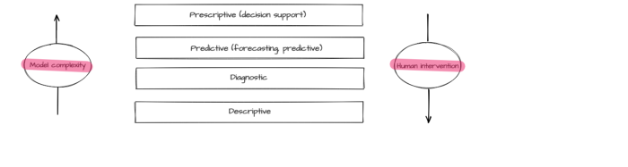
An efficient operation of a complicated technological system requires various analytics and monitoring methods ensuring control, management, and proactive modification of different parameters. Typically, monitoring is executed via different common tools (such as reliable event collection and visualization systems). On the other hand, creating efficacious analytic tools requires additional research, experiments, and excellent knowledge of the subject area. Data analysis methods can be divided into four basic types [1]:
- descriptive analytics visualizes the accumulated data, including transformed and interpreted data in order to provide a view of the entire picture. While it is the simplest type of analysis, it is also the most important type for other analysis methods application;
- diagnostic analytics is aimed at finding the causes of the events that had taken place in the past and at the same time at identifying trends, anomalies, and characteristic features of the described process, its cause, and correlations (interrelations);
- predictive analytics creates a forecast based on the identified trends and statistical models derived from historical data;
- prescriptive analytics recommends the best solution for the task based on predictive analytics, for instance, recommendations on equipment operation and business processes optimization or a list of measures preventing emergency conditions.
Predictive and prescriptive analytic often relies on modeling methods including machine learning. The model effectiveness level depends on the quality of data collection, processing, and preliminary analysis. The forementioned types of analytics differ by the complexity of applied models and by the required degree of human intervention.
There are a lot of spheres where analytics tools can be implemented: information security, banking, public administration, medicine, etc. The same method is often effective for different subject areas. Therefore, analytics system developers tend to create universal modules, containing various algorithms.
Most technological system monitoring results can be represented as time series [2]. The most important properties of a time-series are:
- binding each measurement (sample, discrete) to the time of its appearance;
- equal time-distance between measurements;
- possibility to reconstruct process behavior in current and future periods based on the data obtained in the previous periods.
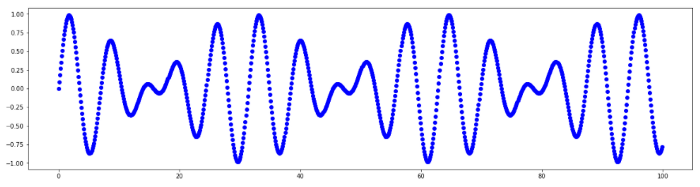
Fig. 1. Time series
Time series capabilities are not limited to numerically measured process descriptions. Using various methods and model architectures, including deep learning neural networks, allows working with data related to natural language processing (NLP), computer vision (CV), etc. For example, chat messages can be converted to numeric vectors (embeddings) sequentially appearing at a certain time, and video is nothing more than a time-dependent numeric matrix.
Time series are handy for describing complex devices operation and are often applied in typical tasks such as modeling, prediction, feature selection, classification, clusterization, pattern recognition, anomalies detection. Use examples include electrocardiogram tracing, change of stocks’ and currencies’ prices, weather forecast value, network traffic volume, engine operation parameters, etc.
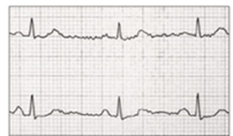

Fig.2. Application examples: electrocardiogram, weather forecast.
There are four time series properties quite accuratly describing its features:
- period — is a period with a constant length within the series and on the ends of which series has close values;
- seasonal — periodicity property (season=period);
- cycle — series characteristic changes due to global circumstances (for instance, economic cycles), there is no permanent period;
- trend — a tendency of time series values to increase or decrease.
Time series may contain anomalies. Anomaly is a deviation in a process standard behavior. Machine anomaly detection algorithms use process operation data (datasets). Depending on the subject area, a dataset may include various anomalies. There are several types of anomalies:
- point anomalies are characterized by behavior deviation in separate points;
- group anomalies are characterized by point group abnormal behavior, yet separately these points are not abnormal;
- contextual anomalies are characterized by connection to external data unrelated to series values (for example, negative outside temperatures during summer season).
Point anomalies are the easiest to detect: these are the points where process behavior differs a lot from other points. For example, a significant parameter value deviation is observed in a separate point.
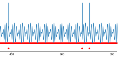
Fig.3. Several point anomalies.
Such values are called outliers. They have a significant impact on the statistical figures of the process, though outliers are easy to detect by setting a threshold for the observed value.
It is harder to detect an anomaly when the process behaves “normally” at every point, but joint values in different points have “strange” behavior. An example of such strange behavior is alternations in signal form, statistical figures (average value, mode, median, dispersion), intercorrelation emerging between two parameters, minor or short-term amplitude anomalous changes, etc. In this case, the challenge lies in detecting parameters’ anomalous behavior undetectable by standard statistical methods.
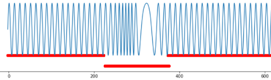
Fig.4. Group anomaly, frequency variation.
Anomalies detection is vital. In one case, we need to cleanse data to get a clear insight, in the other, anomalies should be thoroughly examined as they indicate that the observed system is close to emergency operation mode.
It is very complicated to detect anomalies in time series (unprecise anomaly detection, no labeling, unobvious correlation). Comprehensive state-of-the-art algorithms for detecting anomalies in time series have a high False Positive level.
Some anomalies can be detected manually (mainly point anomalies), if a good data visualization is provided. However, group anomalies are more difficult to detect, especially if there is a significant amount of data and analysis is required for information from several devices. “Anomalies in time” are also difficult to detect since a signal with normal parameters may appear at the “wrong time”. Therefore, for time series, it makes more sense to apply automation to anomalies detection methods.
Anomalies detection in real-life data poses another problem. It is usually unlabeled and, therefore, no initial strict anomaly definition and no rules for its detection exist. Under such circumstances, unsupervised learning methods, where models independently determine interconnections and distinctive patterns in data, are more appropriate.
Algorithms for anomalies detection in time series are often divided into three groups [3]:
- proximity-based methods are used for anomaly detection based on information about parameters proximity or fixed-length sequence parameters, suite for point anomaly and outlier detection but unable to detect changes in signal form;
- prediction-based methods build prediction model and compare their prediction with an original value, work best with time series with expressed periods, cycles or seasonality;
- reconstruction-based methods use reconstructed data pieces; therefore, they can detect both point and group anomalies, including changes in signal form.
Proximity-based methods are intended for detecting values significantly deviating from the behavior of all other points. The simplest example of this method implementation is threshold control.
The main goal of prediction-based methods is building a qualitative process model to simulate the signal and compare the obtained modeled values with the original ones (true). If the predicted and the true signals have close values, then the system behavior is considered “normal”; if the values in the model differ from the true values, the system behavior will be declared anomalous at this segment.
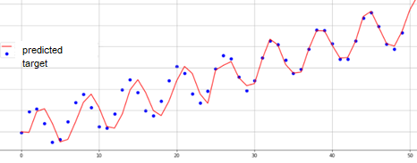
Fig.5. Time series modeling.
SARIMA [4] and recurrent neural networks [5] are the most popular methods for time series modeling.
An original approach is implemented in reconstruction-based models: at first, the model is trained to encode and decode signals from an available selection, while the coded signal has a significantly smaller dimension than the original. Therefore, it is required to “compress” information. An example of such compression for 32×32 pixels pictures to 32 number matrix is represented below.
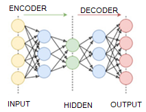
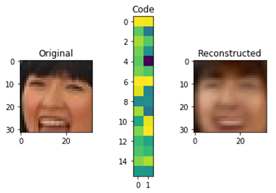
Fig.6. Autoencoder operation scheme.
After the model training is complete, segments of the examined time series are used as input signals. If encoding-decoding is successful, the process behavior will be considered “normal”; otherwise, its behavior will be deemed anomalous.
One of the recently developed reconstruction-based methods is TadGAN [3] which has achieved impressive results on anomalies detection. It was developed by MIT researchers at the end of 2020. TadGAN method architecture contains an autoencoder and a generative adversarial network elements.
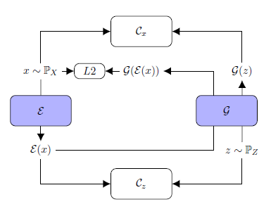
Fig.7. TadGAN architecture (from article [3])
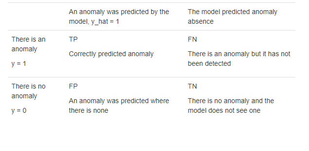
Ɛ acts as an encoder mapping x time series sequences into z latent space vectors, and G is a decoder, reconstructing time series sequences from a latent representation z. Cx is a critic, evaluating G(Ɛ(х)) reconstruction quality, and Cz is a critic evaluating z = Ɛ(х) latent representation similarity to white noise. Besides, “similarity” control of the original and the reconstructed samples is applied using L2-measure based on “Cycle consistency loss” ideology (ensures common similarity of generated samples with the original samples in GAN) [6]. The resulting target function is a sum of all metrics intended to evaluate the quality of Cx, Cz critics operation, and the original and the reconstructed signals similarity measures.
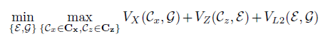
Various standard high level API packages (e.g. TensorFlow or PyTorch) may be used to create and train neural networks. In the repository [7], you can find an implementation example of an architecture similar to TadGAN, where the TensorFlow package is used for weights training. During model training five metrics were optimized:
- aeLoss — mean square deviation between the original and the reconstructed time series in other words a discrepancy between x and G(Ɛ(х)),
- cxLoss — the Cx critic binary cross entropy, determining difference between the original time series segment and the artificially generated one,
- cx_g_Loss — binary cross-entropy, a G(Ɛ(х)) generator error, characterizing its incapability to “fool” the Cx critic,
- czLoss — the Cz critic binary cross-entropy, determining the difference between latent vector generated by the Ɛ encoder and white noise, ensures Ɛ(х) latent vector similarity with a random vector preventing the model to “learn” separate patterns in the original data,
- cz_g_Loss — binary cross-entropy, a Ɛ(х) generator error, characterizing its incapability to create latent vectors similar to random ones and thereby “fool” the Cz critic.
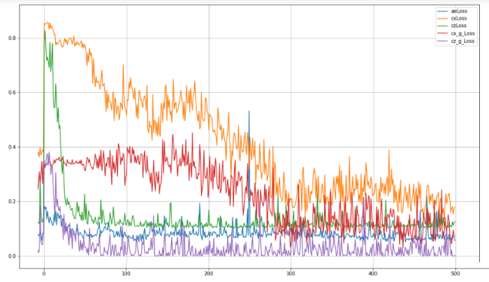
Fig.8. TadGAN model training quality for 500 epochs.
After the model training is complete, reconstruction of separate segments belonging to explored time series is executed; original and reconstructed series are to be compared by one of the following methods:
- point by point comparison;
- curve areas comparison in a field around each sample (width is a hyperparameter);
- Dynamic Time Warping [9].
Binary classification problem quality is evaluated through F1-metric: “positive” (zero hypothesis) — there is an anomaly; “negative” (alternative hypothesis) — there is no anomaly.
To demonstrate how the method works, we will use synthetic (artificially created) series without anomalies. This series is a sum of two sinusoids which values vary in the range from -1 to 1.
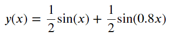
The series curve:
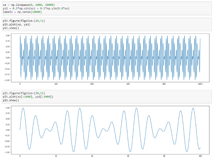
Fig.9. Synthetic series graph.
The series reconstructed by TadGAN for a various number of stages (4 and 80) will be as follows:
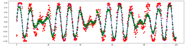
Fig.10. Series modeling by TadGAN for a different number of epochs (4 epochs — red, 80 epochs — green).
We can see that the model has learnt to predict main patterns in data. Let’s try addiing various anomalies in data and then detecting them by the TadGAN model. At first, we are going to add a few point anomalies.
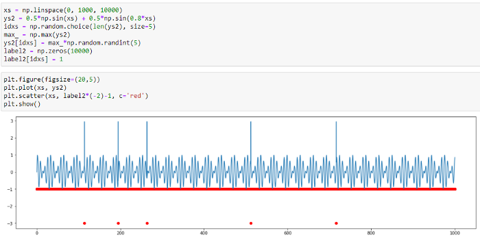
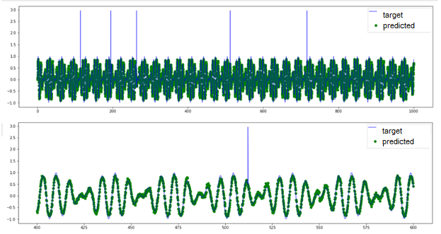
Fig.11. Point anomaly detection by TadGAN
Based on the original and the predicted signal curves, we can see that the model cannot reconstruct anomalous value “peaks”; however, it can detect point anomalies with high accuracy. In this case, it is difficult to see what benefit we gain using such a sophisticated model as TadGAN because similar anomalies can be detected by the threshold exceeding evaluation.
And now, let’s turn to a signal with another anomaly type: periodic signal with anomalous frequency variations. There is no threshold exceeding here. All series elements have “normal” values from the perspective of amplitude, and the anomaly is detected only in the group behavior of several points. TadGAN is also incapable to reconstruct a signal (as you can see in the picture) and cannot be used as evidence of a group anomaly.
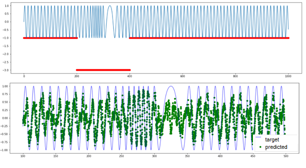
Fig.12. Results TadGAN operation on a dataset with anomalous frequency variations.
These two examples illustrate how the method works. You can try creating your own datasets and check the model capabilities in various situations.
More complicated dataset examples were published by the TadGAN developers in their article. There is also a link to another MIT specialist development — the Orion library, capable of detecting rare anomalies in time series applying the unsupervised machine learning approach.
As a conclusion, there is a lot of various comprehensive anomaly detection methods implementing signal reconstruction (reconstruction-based); for instance, arxiv.org contains dozens of articles describing various modifications to the approach, implementing autoencoders and generative adversarial networks. It is highly advisable to choose a specific model for each problem considering its requirements and subject area.
The technology described in this article has practical application in CL Thymus, CyberLympha’s AI/ML-based software, designed to protect OT networks and Industrial Control Systems that operate data exchange protocols based on unknown or proprietary protocols with no specifications available to the public. More info about CyberLympha and its products is available on the company website.
References
- “What is a data analytics?” (ru), https://www.intel.ru/content/www/ru/ru/analytics/what-is-data-analytics.html
- Dombrovsky. “Econometrics” (ru). http://sun.tsu.ru/mminfo/2016/Dombrovski/start.htm
- “TadGAN: Time Series Anomaly Detection Using Generative Adversarial Networks”, https://arxiv.org/abs/2009.07769
- “An Introductory Study on Time Series Modeling and Forecasting”, описание SARIMA https://arxiv.org/ftp/arxiv/papers/1302/1302.6613.pdf
- Fundamentals of RNN, https://arxiv.org/abs/1808.03314
- Cycle Consistency Loss, https://paperswithcode.com/method/cycle-consistency-loss
- https://github.com/CyberLympha/TadGAN
- Orion, a library for anomaly detection, https://github.com/signals-dev/Orion
- Dynamic Time Warping algorythm description, https://towardsdatascience.com/dynamic-time-warping-3933f25fcdd
- https://medium.com/mit-data-to-ai-lab/time-series-anomaly-detection-in-the-era-of-deep-learning-dccb2fb58fd
- https://medium.com/mit-data-to-ai-lab/time-series-anomaly-detection-in-the-era-of-deep-learning-f0237902224a
- Of Physics and Poetry
In all fields of science, simplifying the real world in order to successfully develop various theories for the imaginary world is quite normal. Physicists have a full set of artifacts: a perfect gas, a point mass, a perfectly rigid body, an ideal fluid, etc.
And it works! Perfect gas law describes real gases quite well, and classical mechanics successfully deals with motion calculus for bodies of different size (as long as we stay out of quantum world or vice versa as long as body masses don’t fall under general relativity theory).
A smart way to call such process is model reduction. In other words, we simplify a real system to the max, then develop a mathematical model that is capable of predicting system behavior and then — boom! — it just so happens that the real system complies with the discovered regularities.
Similar method is also applied in information security. Today we will review one of such artifacts — a restricted software environment and how this environment helps solving real problems of establishing required information security level in real systems.
2. How Security Modeling Turned Into Science
But first things first: let’s talk about historical background. In the 1970s, a really important event for information security sphere occurred. The United States Department of Defense bought a computer. Something like this:
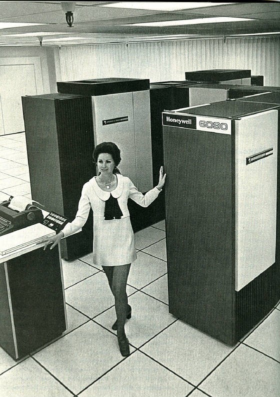
Honeywell-6080 mainframe. A girl on the photo is either an eye stopper or to help understand the scale…
Since it was many moons ago when trees were small and computers were huge, the Department of Defense had enough money (or, maybe, space) just for one computer. Naturally, they planned to process some secret data with its aid. However, at that moment the predecessor of Internet — ARPANET — had already existed and the Department of Defense apparently did not want to limit themselves to working with secret data but also felt like researching some funny cat pictures…
Consequently, a wild challenge appeared: how could one make processing classified and non-classified data on the same mainframe possible? Moreover, a multi-user environment was required and intended end-users were to be of two types: department officers and civilians from ARPANET (and it is well known by militaries that civilians cannot be trusted at all).
That was how Project №522B started. It was a research and development project intended for… Well, judging by the results, its main goal was to create an academic discipline named “Theoretical Foundations of Computer Security”, describing almost every security approach used in modern software.
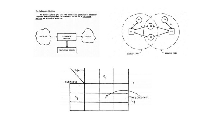
Screenshots of Project 522B original reports: reference monitor, security domains and access matrix. These are just a small part of theoretical conceptions developed within the framework of this project.
A separate article could be written about the results of Project 522B research as well as about its participants who became legends in the world of information security. However, at this time our interest is limited to a specific topic which is a subject-object integrity model.
3. Subject-Object Integrity Model in Plain English
So, we have made a decision, that in order to develop a theoretical system model that can be useful for solving the security problem, we need to simplify the initial system somehow.
The simplification has been easily found. Let’s consider the whole system as a collection of subjects (i.e. active entities e.g. processes) and objects (i.e. passive entities e.g. data files). Subjects will somehow interact with objects e.g. carry out access (or create information flow). We will divide all access options (a P set) into authorized access (PL) and unauthorized access (PN).
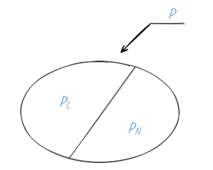
Yet, this model is oversimplified… How about bringing it a little bit closer to reality?
- Subjects can appear and disappear as different processes can be started and stopped in computer systems. At the same time, a subject can not appear out of a clear blue sky: in real systems a subject (an executable file, a script etc.) is created out of some data previously contained in the system i.e. there’ll always be an object at the beginning.
- Objects can affect subject behavior, for example, if the object is an application configuration file.
- Objects can be changed (subjects gain access to objects for some reason, let’s say they change something).
- A special subject (let’s name it a reference monitor) has to monitor compliance with access control policy (i.e. ensure that each access belongs to PL).
- A security monitor also has related objects (that contain PL description), that are affecting its operation.
And to make it harder, let’s mention that access operations when subject S accesses object O at t1 and t2 points in time are, in fact, two different access operations because in the timespan between t1 and t2 both subject S and object O might have changed. Consequently this makes describing P set quite challenging because it contains an infinite number of elements!
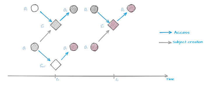
Subject S1 gains access to object O2 at t1 and t2, but now they are totally different object and subject…
So, how can we ensure that only access operations that belong to PL are permitted in this chaos if we can’t even describe PL itself?
For starters, let’s take a closer look at objects affecting subject’s behavior (i.e. executable files, configuration files etc.). Let’s say we have 2 subjects and we know all objects affecting these subjects’ behavior. Such objects are called associated with the subject.
If we can ensure that each subject can not gain access (or create an information flow) to objects associated with its neighbor, then we can call such subjects correct with respect to each other. If sets of objects associated to each of these subjects have no intersection then we can call them perfectly correct with respect to each other.

Using this definition, we can develop a criteria for a guaranteed implementation of the access policy in the system: if at the initial point in time all subjects are perfectly correct with respect to each other and they can perform access operations (generate flows) that belong to PL only, then over time they will be able to perform access operations from PL only. Such set of subjects is called a perfectly restricted set of subjects.
So, here is what looks like a perfect solution for the task! Only it’s not. In fact, this means that, for example, each user in a multi-user system works on his or her own isolated computer that can’t interact with a neighbor’s computer. What a splendid multi-user system that allows information exchange via users only…
I won’t make you suffer through mathematical subtleties so let’s cut the chase and go straight to the solution that will allow the implementation of the restricted software environment in real life rather than in vivid imagination of a security theorist.
Let’s add another security capability to our model and assume that creation of a new subject S out of object O is possible only if object O has not been changed since the initial moment in time (it’s called “creation of a subject with integrity control”). This small change can make a big difference:
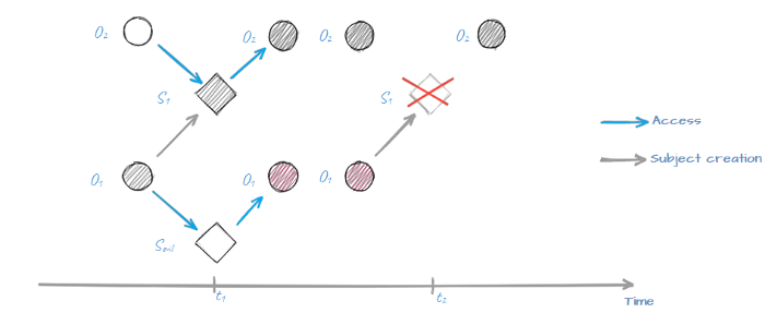
The sequence was broken because object O1 has changed at t1 making the creation of the modified subject S1 impossible
The most important change is that we have guaranteed a finite amount of subject variations in the system regardless of its operation time. After all, we have a limited set of objects that can be used for subject creation.
This difference helps us to come up with a sensible access control algorithm.
We can describe the PL set for all subjects and all objects in such a way as to ensure correctness with respect to each other for all subjects (it is important to note that we are not talking about perfect correctness, therefore multiple subjects can be created from a single object). This set is finite because the amount of objects is finite at the initial point in time, and so is the set of created subjects. And we can be sure that as time passes nothing will change: there will be no new subjects that would be able to get around the limits of the security monitor and rewrite our policy because creation is performed with integrity control.
All we have left to do is make sure that this approach can actually be transferred from mathematical description to real system capabilities while keeping the obtained system security property. Let’s get it done.
4. Restricted Software Environment in Real Life
First, we’ll try to solve the problem described by the US Department of Defense (although we’d be half a century late). In order to make multiple users able to work with a single mainframe securely, we need:
- An operating system component which will control the integrity of the software executable file prior to running it. If the integrity check fails — the software would not be permitted to run.
- An access control policy (e.g. in a form of an access control matrix) which will outline which software would have access to which files (most importantly write access, as our main problem is protecting the system operation algorithm from any modifications that would allow system security policy violation). Our primary concern is software executable files (and operating system kernel components) as well as various data files that affect software operation algorithm.
Everything works as long a we have a single computer. Things get complicated when we consider a modern system that consists of multiple components connected to each other via a local network. Sure, we can always go hardcore and configure both local and network access control by using IP mechanisms such as CIPSO option (by the way, this is another interesting topic which I could cover if you’re interested), however, it’s technically impossible for a heterogeneous network.
Therefore, we will set a few technical restrictions on a real system and see whether they coincide with theory in terms of restricted software environment:
- We can control subjects’ integrity. Though not every creation can be stopped even if integrity check fails (how can we stop a network switch from loading its software even if we discover that its startup configuration has been modified?).
- It’s not always possible to control separate processes’ access to objects. That same network switch has a firmware that contains multiple processes accessing various objects (files, separate records, device-specific data, such as CAM-tables, etc). However, this switch has no standard mechanism for setting any access control matrix for these subjects and objects.
- We can’t control subjects’ access to objects located within other network nodes. In fact, it might be theoretically possible. Carry all interaction through a firewall, do a thorough traffic inspection, apply a strict interaction control policy similar to access control matrix… But in the real world things won’t work this way. This firewall will require tremendous computing resources and it’s admin would have to be extremely patient in order to configure this setup.
And so, how can we solve the problem, considering all these limits?
First of all, integrity control should not be omitted: executable files, configuration files (or more complicated objects such as databases, registry keys or LDAP catalog objects) can be controlled both locally and remotely via the network.
Second, we should divide all interactions into two classes: when subjects and objects are within the node, and when subjects and objects are network nodes themselves. Network node “integrity control” would encompass the permanence of the nodes’ list and their network properties (address, name, open ports, etc).
Third, we can replace the access control matrix for subjects and objects with network flows detection and monitoring (in this case they represent the data flows between subjects and objects). Assuming that at the initial instance (which could also be a continuant interval) all accesses (flows) in the system belong to PL set, we can set them as legitimate and consider any detected flow that does not belong to the set, formed at the initial instance, a violation. However, we should always bear in mind that this assumption is valid only for the systems operating under a single algorithm (or a set of very similar algorithms). For this reason, restricted software environment model is good for all kinds of cyber-physical systems but is hardly applicable for a typical “office” network that sees a lot of changes every minute.
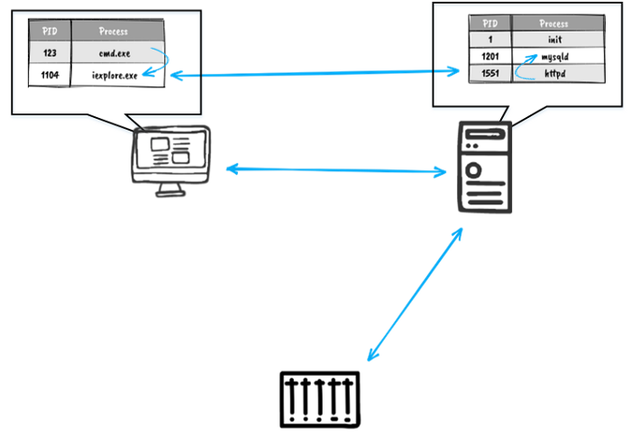
Two-level subject-object model. The first level deals with information flows between network nodes, the second level deals with processes interactions inside each network node.
Let’s summarize what we’ve discussed. Implementation of restricted software environment is a good way to ensure security of different cyber-physical systems (where integrity is one of the most important properties of information).
Establishing restricted software environment for this type of systems can be performed by correct security mechanisms settings applied to each network node as well as via deploying a dedicated device capable of the following:
- Maintaining a database of network objects and their network parameters.
- Monitoring objects’ modifications (i.e. configurations, executable files etc.). In particular, reference monitor configuration on each device should be monitored.
- Control information flows between the nodes and generate alarms upon detecting an unknown flow (since the probability of this flow belonging to PN set is quite high).
And so, we have successfully obtained a list of main capabilities of the ICS Asset Management solutions class. Coincidence? I don’t think so…
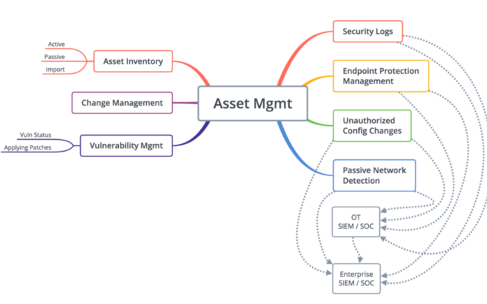
Capabilities of ICS Asset Management solutions according to Dale Peterson
A lot of solutions that belong to ICS Asset Management and Detection class are available on the market today but their basic capabilities are often very similar. And now you know why. The technology described in this article has practical application in the CL DATAPK software, CyberLympha’s flagship product, focused on securing enterprise Industrial Control Systems and OT infrastructures. More info about CyberLympha and its products is available on the company website.
1. Relevance
Modern plants, as well as large trains and ships, use data transmission networks. Most of the time this data is quite critical and consequently worth protecting. The market offers quite a few network security tools and solutions but in order to use them it is important to know what kind of hosts operate on this protected network, what are their addresses, and how do they interact with each other.
In this article, we’ll focus on one of the methods used to identify network hosts type by a trendy machine learning algorithmn.
One could certainly think that there are numerous tools (including Nmap — one of the most well-known) for network host class remote identification. What’s the point in re-inventing the wheel, right? The thing is, popular tools generally use active scanning and this is not something we’d desire to happen in the industrial network. Whatever good intentions it may have, an annoying scanner is constantly polling hosts and consequently can cause PLC failure (each additional unnecessary packet is a reason for PLC to freeze or reboot).
What’s more, available tools are designed for allocating the network hosts to a limited class set, based on some predefined rules. Any object, that was not explicitly covered by the ruleset, stays unindentified. The method we’re going to cover here is free of this limitation. As a bonus, it facilitates both inventorizing your assets and identifying anomalies in hosts’ information exchange flows.
If, for some reason, using active scanning tools is impossible, one has to resort to manual host identification and description (no choice here, we’ve got to know what assets need to be secured). To automate this we can utilize a method for host class identification based on an observed network traffic profile. This method does not require any interaction with the network and ensures protected system integrity.
2. The idea
This method is similar to IDS operation principle: intercept and store all traffic. Next, divide the traffic into flows — connections between hosts with unique addresses that use a unique set of different level network protocols. Next, count how often a host uses one or another protocol set and generate a feature vector out of these numbers. Finally, choose an optimum model architecture using marked hosts from a training set and AutoML methods, and train it afterwards.
The trained model receives feature vectors of the unindentified hosts, and as an answer, we obtain their assumed types. That is it, all hosts are identified and allocated.
Detecting anomalies takes even less data. Using the described method to generate a feature vector for each host. Since we apply a supervised learning algorithm (allocation to classes is unknown in advance), we will need to determine an optimum number of clusters and divide hosts among them. Using cluster numbers as answers, we can train a neural network with the available data. In subsequent operation, new flows detection will require updating the hosts’ feature vectors and predicting their classes with the neural network. If the class matches the one previously known — do nothing; otherwise [ring the alarm, we are under attack!] register an anomalous activity for the host. In order to determine the severity of the event, we can apply hierarchical clustering additionally to custom clustering when dividing hosts into groups. Subsequently, we can indirectly define event severity by cophenetic distance (distance from one node to another in the hierarchy). For example, an appearance of a new client of the file server and a new management flow to a switch, a flow which has never been detected before, are events with quite different severity levels.
3. The math (formal model)
Sometimes mathematics is called a universal language of science. Let’s try and translate the idea of network host class identification and make some parts more specific.
The model takes protected system network traffic as its input. Let’s name a set of network packets using the same protocols in every network layer involved and sent from one network address to the other a flow. A vector of characteristic
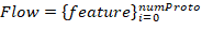
describes Flow, where it’s length numProto depends on the number of the network protocols in the packet.
Therefore,
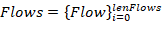
characteristic set describes the entire flow set Flows with length lenFlows:
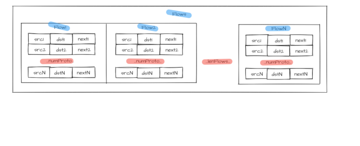
Figure 1 — Flow group
Source addresses set is used with all numProto network model layers as an identifier for each host from allocated hosts array Hosts with length lenHosts.
Addressing levels number numProto reflects the number of the nested protocols:

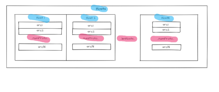
Figure 2 — Hosts identifiers
The main characteristics for each host include relative flows number hosts.num_flows and protocols used in these flows. For each host,

vector of characteristics is described. Its length host.numKnownProto matches the total number of identified protocols (all layers) in the entire flow array. A number from 0 to 1 characterizes each frequency element and depends on the number of host flows containing a respective protocol.
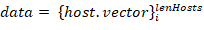
A host has a
label set. Each set describes a host belonging to one of the classes. Class groups are formed independently by two attributes: host role (i.e. PLC, Workstation, Active network hardware,…), operating system (Windows XP, Windows 7, Linux Ubuntu, Linux CentOS, …).
Another characteristic of each host is the proportion of flows linking it to hosts belonging to specific classes host.connectedWith.
To make the host description suitable for the machine learning models essential characteristics are set as a host.vector host characteristic vector. We can also add other information about the host in form of the host.some_inf. This vector combined with information about protocols usage frequencies constitutes host.vector = {host.proto,host.some_inf} host traffic profile or characteristic vector.
Source data
for a model is represented as a hosts characteristic vectors set. Prior information about hosts classes is required to train a model; therefore, it is necessary to set each

This means that the traffic dump should contain flows that correspond with all input data (sources addresses for each hostᵢ host), where the answer is known in advance — label host type.
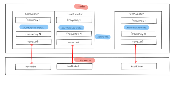
Figure 3 — Source data for model training
Available traffic with labeled hosts is divided into two parts: one for training and another for testing. First, the model is trained on the training set with host.label parameter values as answers known for all hosts. Then the model identifies hosts from a test set. Selected metrics will assess the model operation quality after comparing predicted host.labelPredicted and host.label prelabeled classes. If it meets the specified requirements, the model is saved, otherwise, model structure or its hyperparameters undergo changes, and the training cycle (training, testing, and model changing) repeats until the model makes predictions with sufficient quality.
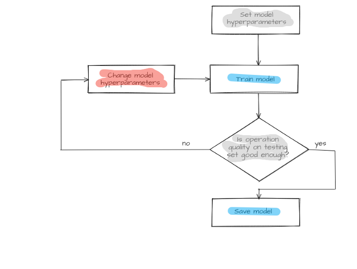
Figure 4 — Model creation process
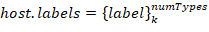
And now let’s switch to the second task: anomalies detection in network traffic. Here the characteristic vectors should be selected from the flow set. They are to be divided into groups through clustering models. Each host will get a class according to its group number. Consequently, the entire multidimensional space, with dimension equal to characteristic vector length, will be split into multiple domains. The number of the domains will be equal to the number of clusters.
Concurrently, the hierarchical clustering model is used for cluster analysis. It will form a division saved for use during the next step.
When a new Flows flow group appears, host.vector host characteristic vectors will be updated and sent to the model input. Model operation results are saved in a respective host property host.new_label and compared to host.label known host clusters. If there is a discrepancy (hostᵢ.label ≠hostᵢ.new_label) it will be considered an anomaly. Flows flows that have led to this discrepancy (flows that changed host characteristic vector host.vector) are considered anomaly initiators. An operator will get an alert concerning potentially dangerous flows and host host specifications for the host that has displayed anomalous behavior. Hosts division formed by the hierarchal model is used to determine severity. The severity of a host moving from one group to another equals cophenetic distance between an anomalous host and its new nearest neighbor.
If there are no discrepancies between already known and newly received classes (hostᵢ.label = hostᵢ.new_label) the model will train again. In this case, hosts’ updated (multidimensional space undergoes re-layout) characteristic vectors host.vector are used as input data. Subsequently, the model goes into standby mode while waiting for the next flow set. A new hierarchical division is also formed. It is deemed that this time no anomalous behavior has been detected.
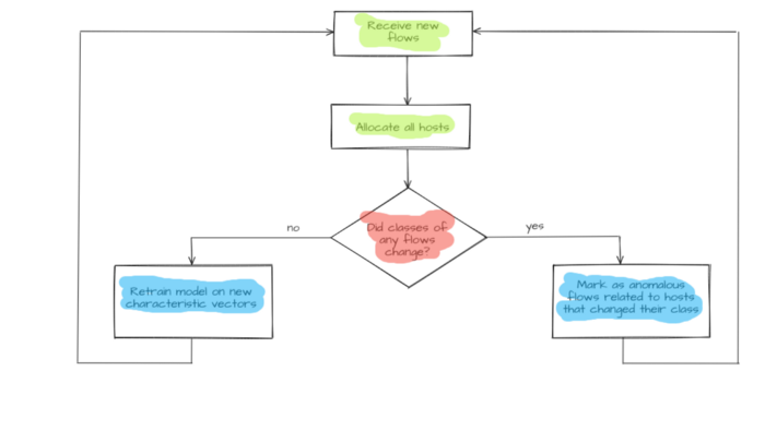
Figure 5 — Anomalous flows detection
The described formal model helps determine classification features and detect anomalies in hosts behavior.
4. Model implementation
The traffic flows were collected using the DPI module of the CyberLympha DATAPK product. Characteristic vectors were formed from these flows by a Python script.
One of the ways to choose an optimal model architecture is to use an automated machine learning method TPOT offered in TPOT module for Python.
As a result, we have designed a two-block ensemble that is united by stacking method. The first block includes K-neighbor models united by the stacking method as well. Answers given by lower layer models are additional features for upper layer models.
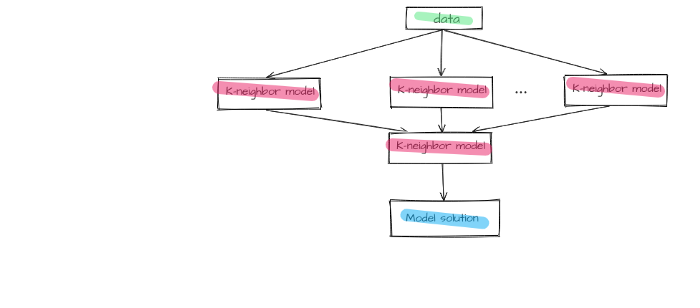
Figure 6 — First block of the final model
The second block includes a naive Bayes classifier model with minimum smoothing.
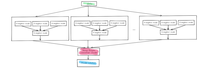
Figure 7 —The final model
The chosen model is implemented by means of the sklearn library.
Anomaly discovery is handled by the DBSCAN method for initial clustering, the SciPy library for hierarchical clustering, and a neural network for hosts allocation to the groups.
5. The results
So far, the available data is insufficient for estimating the accuracy of the module operation. It is still too soon to talk big about the numbers achieved until the product reaches the phase of field testing. During test sessions using available data (other than in the training set) F1- measure accuracy reached 80%. A loophole was implemented for situations when the model is unsure about the decision. In this case, it is acceptable to offer the choice between the two most probable classes to the end user. This allows F1 measure to increase up to 95–98% however if we compare the amount of such cases to the total set we can clearly see that they are rare. Therefore, this option can be considered worthy.
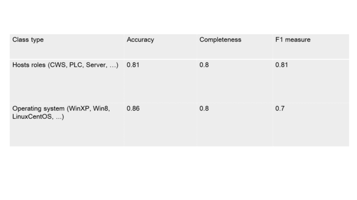
Table 5.1 — Classifier operation accuracy
We are going to consider a confluent though simple and understandable example to demonstrate capabilities.
Let’s assume that four active hosts operate in an enterprise network: a PLC, a SCADA, and two workstations (CWS). In this scenario the PLC interacts with the SCADA-server via Modbus (Ethernet, IPv4, and TCP at lower layers), the SCADA interacts with the workstation №2 via HTTP with the same lower-level protocols set, and with workstation №1 via SSH.
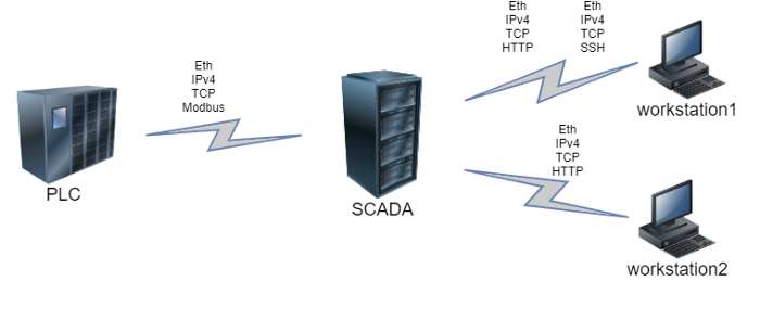
Figure 8 — Flows diagram
Let’s make a table containing protocols usage frequency by each host at each OSI layer:
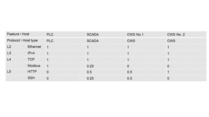
Table 5.2 — Protocol usage frequency by hosts
Now we can set a vector for each host according to the table above:
PLC = [1, 1, 1, 1, 0, 0]; SCADA = [1, 1, 1, 0.25, 0.5, 0.25];
CWS №1 = [1, 1, 1, 0, 0.5, 0.5]; CWS №2 = [1, 1, 1, 0, 1, 0]
You can see that the vector elements are the same for all classes. For this reason, we are not going to take them into account during model training. The last elements are the most important here.
Let’s save the vectors:
samples = [
[1, 1, 1, 1, 0, 0],
[1, 1, 1, 0.25, 0.5, 0.25],
[1, 1, 1, 0, 0.5, 0.5],
[1, 1, 1, 0, 1, 0]
]
And true classes for each example:
answers = [
‘PLC’,
‘SCADA’,
‘CWS’,
‘CWS’
]
Based on the support vector machine, we are going to create a simple model (the examples number is insufficient for the described model to learn).
from sklearn import svm
model = svm.SVC(kernel=’poly’, degree=3)
model.fit(samples, answers)
Now it’s time for our model to operate with new data. Let’s assume that we’ve added another workstation to the network. However, this workstation will differ from the previous two. It’s sole purpose will be SCADA-service control and it will only generate flows that use SSH protocol. Here’s an updated network scheme.
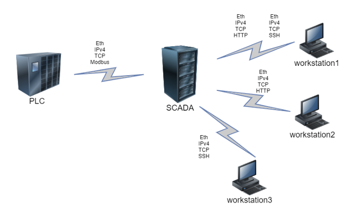
Figure 9 — New flows diagram
A new host requires one more feature vector, and the feature vectors for the existing hosts, that interact with the new node are bound to be updated. In this case it is the SCADA: usage frequency increases for SSH and decreases for other protocols.
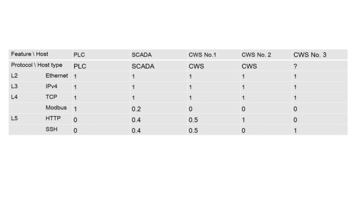
Table 5.3 — Protocols usage frequency by hosts after adding a new host
Let’s set a vector for the target host: CWS 3 = [1, 1, 1, 0, 0, 1];
unknown_node_vector = [
[1, 1, 1, 0, 0, 1]
]
And let’s see the prediction, given by the model we trained earlier:
model.predict(unknown_node_vector)
>>> array([‘CWS’], dtype=’<U5')
You can see that the model has generated the correct answer. In real life the service uses more hosts, each of them having more features, but the given example illustrates the operation concept quite well.
6. The reality
Currently, the described service exists only as a prototype. However, if and when it goes into release, there’s no doubt that security departments working at the plants and ships mentioned in the beginning, will save a lot of time on manual host type detection and assignment. Consequently the security personnel will be able to focus on non-trivial tasks, increasing the security level of company assets.
The technology described in this article has practical application in CL Thymus, CyberLympha’s AI/ML-based software, designed to protect OT networks and Industrial Control Systems that operate data exchange protocols based on unknown or proprietary protocols with no specifications available to the public.
GISEC-2021 upcoming global cybersecurity event is scheduled to take place in Dubai World Trade Center on May 31 – June 2
We see this as a perfect opportunity to join in with the international cybersecurity community and begin offering our products and services on the global market. A live demo will be available at our booth, and we’ve also prepared an exciting interactive experience for those who wish to get acquainted with CL DATAPK and its benefits. You can find us at booth P10 in the Startup Area of the exhibition. Ivan Ustylenko, Company’s deputy CEO will also be talking about our vision in the pitch session on the Dark Stage on June 2, starting at 10:30.
“Participating in GISEC-2021 is going to be our first global offline exhibition experience. We’re looking forward to entering global community and meeting potential Customers, business and tech partners. I strongly believe this expo will be a great first step for CyberLympha on the international market”,- shared Ivan.

CyberLympha took part in Tech Export to India acceleration program initiated by Moscow Export Center and Global Venture Alliance in the fourth quarter of 2021 The Company has been selected among 30 other nominees from more than 200 applicants, due to CL DATAPK solution maturity and general cybersecurity relevance on the Indian market. The assessment conducted by the experts has qualified CyberLympha products as ready for entering the highly competitive global market. During three months of intensive lectures, master classes and mentoring sessions given by recognized business mentors and industry professionals from both India and Russia, CyberLympha has held multiple online meetings with potential local Customers and Partners, received feedback from over 30 local cybersecurity experts and investors, and conducted a series of interviews with CISOs and professionals working in OT/ICS cybersecurity. Among other project results CyberLympha has developed a working strategy for entry to the Indian market and identifying potential strategic partners. Ivan Ustylenko, Нead of the International business unit, specified that several partnerships agreements are on the way and CyberLympha is looking forward to fruitful collaboration with local Partners and Customers.